Elevation Contour Plots With D3

Creating contour plots of elevation and topography in D3 is challenging due to the availability and format of the data. Most city or county open data websites do not provide topographical data and, when it’s present, elevation data is usually not in GeoJSON or TopoJSON format (unlike many other mapping data sources).

In this post, I’ll show how to acquire elevation data and visualize it as a contour plot in D3. As an example, I used this technique to visualize the topography of my hometown.

folsom topography

Acquiring the Data #

Elevation data is most commonly found in the GeoTIFF or DEM formats. Unlike GeoJSON and TopoJSON, which most D3 users are more familiar with, GeoTIFF and DEM are raster formats. This means that they are a fixed resolution: for example, a raster resolution of 90m means that there is one elevation value (pixel) for each 90m^2.

The best source of topography data I have found is the Shuttle Radar Topography Mission (SRTM), which contains high-resolution topography data of the entire world captured by a space shuttle mission. It can be accessed online, and comes with a very nice interface to select a specific region to download elevation data for:

opentopograpy interface

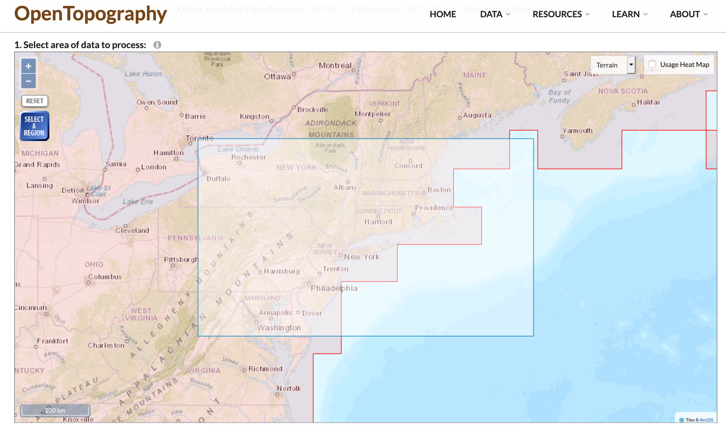
I downloaded the elevation for my hometown as a GeoTIFF. The downloaded file can be inspected online using geotiff.io.

Creating the Plot #

Setup #

First, set up some boilerplate in an HTML file. In addition to D3, we’ll need to import the geotiff library to load our data.

<html>
<script src='https://d3js.org/d3.v7.min.js'></script>
<script src='https://cdn.jsdelivr.net/npm/geotiff'></script>

<body>
    <div id='vis'></div>
    <script>
    </script>
</body>
</html>

Inside the script tag, add an async function so that we can use await in our code. We will write all of the Javascript code to load the data and render our chart in this function.

async function renderVis() {
    // all vis code goes here
}
renderVis();

Loading and Scaling the Data #

To start off, we will load our data and extract the width, height, and elevation values.

let tiff = await d3.buffer('elevations.tif')
    .then(buffer => GeoTIFF.fromArrayBuffer(buffer));
let image = await tiff.getImage();
let rasters = await image.readRasters();
let values = rasters[0];
let w = image.getWidth(), h = image.getHeight();

We’ll need to calculate a scaling factor to fit the visualization to the page. The following code snippet calculates a scaling factor so the visualization takes up 90% of the width or height of the window. The variables width and height will be the dimensions of the final visualization, while w and h are the dimensions of the original GeoTIFF.

let scaling = Math.min(window.innerWidth * .9 / w, window.innerHeight * .9 / h);
let width = w * scaling, height = h * scaling;

Drawing the Contours #

Now that we know the dimensions of the our elevation data, we can add an SVG to the page.

let svg = d3.select('#vis').append('svg').attr('width', width).attr('height', height);

We will use d3.contours to generate the contour shapes for our plot. Note that the dimensions passed to the size function must be the original image size. We’ll also set up a color scale. Feel free to experiment with different color palettes.

let contours = d3.contours().size([w, h]);
let contourData = contours(values);

let colorScale = d3.scaleSequential(d3.extent(values), d3.interpolateViridis);

Now, we can draw the contour plot. Note that we upscale the drawn contour shapes based on our scaling factor.

let path = d3.geoPath();
svg.selectAll('.elevations')
    .data(contourData)
    .join(enter => enter.append('path')
        .attr('class', 'elevations')
        .attr('fill', d => colorScale(d.value))
        .attr('stroke', 'black')
        .attr('stroke-width', 0.1)
        .style('opacity', 1)
        .attr('d', d => path(d))
        .attr('transform', `scale(${scaling})`)
    );

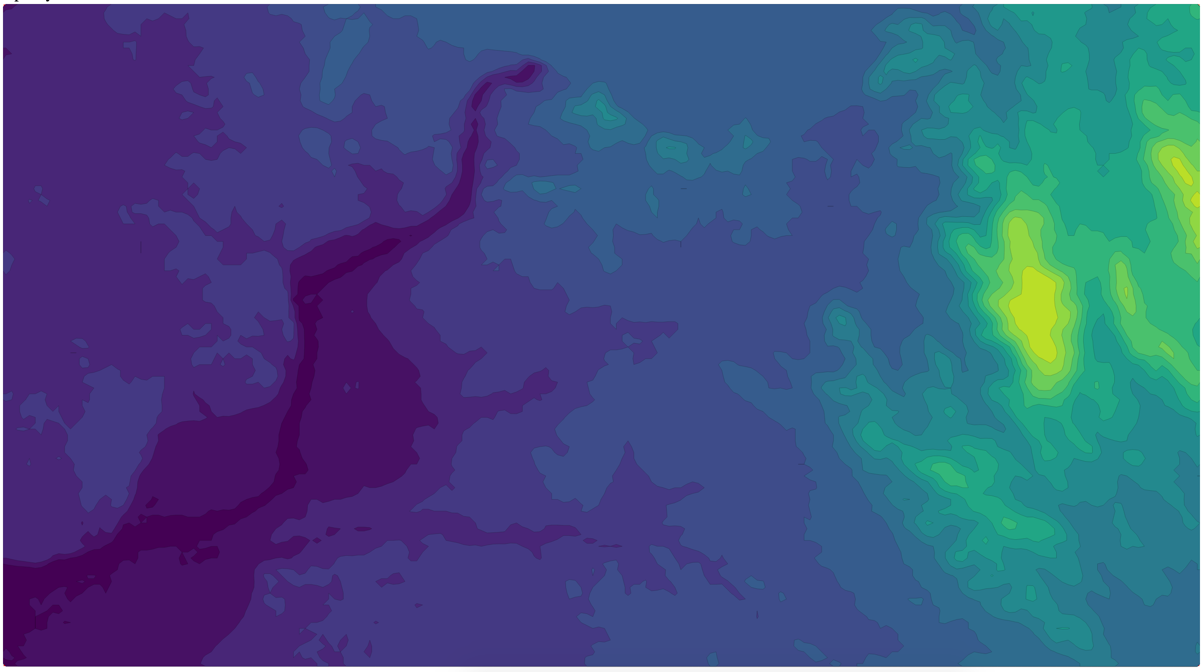
We can load the chart in your browser by placing your HTML file in the same directory as your GeoTIFF file, starting a local http server in that directory using Python (python3 -m http.server), and navigating to localhost:<PORT_NUMBER> in your browser. Using the same data as my example, the chart should look something like this:

example 1

Adding a Legend #

We can add a legend for our chart using the d3-legend library. First, we’ll need to import the library and increase the size of our SVG to fit the legend.

Add the import at the top of the page:

<script src='https://cdnjs.cloudflare.com/ajax/libs/d3-legend/2.25.6/d3-legend.min.js'></script>

We’ll put the legend below the chart, so we’ll have to make a slightly larger SVG.

let svg = d3.select('#vis').append('svg').attr('width', width).attr('height', height + 150);

The library makes adding the legend easy. Feel free to experiment with different orientation, positioning, and styling.

let legend = d3.legendColor()
    .scale(colorScale)
    .orient('horizontal')
    .shapeWidth(50)
    .title('Elevation (m)');
svg.append('g')
    .attr('transform', `translate(10,${height + 25})`)
    .call(legend);

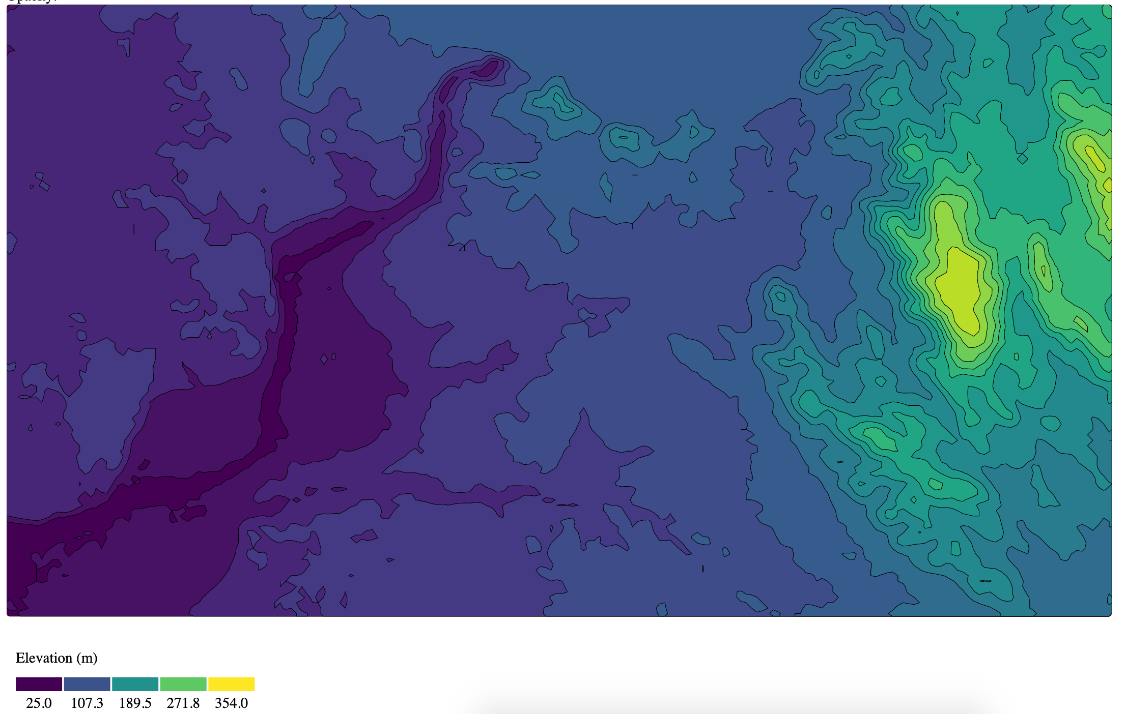
And with that, we’re done! The final outcome should look like this:

example 2

What’s next? #

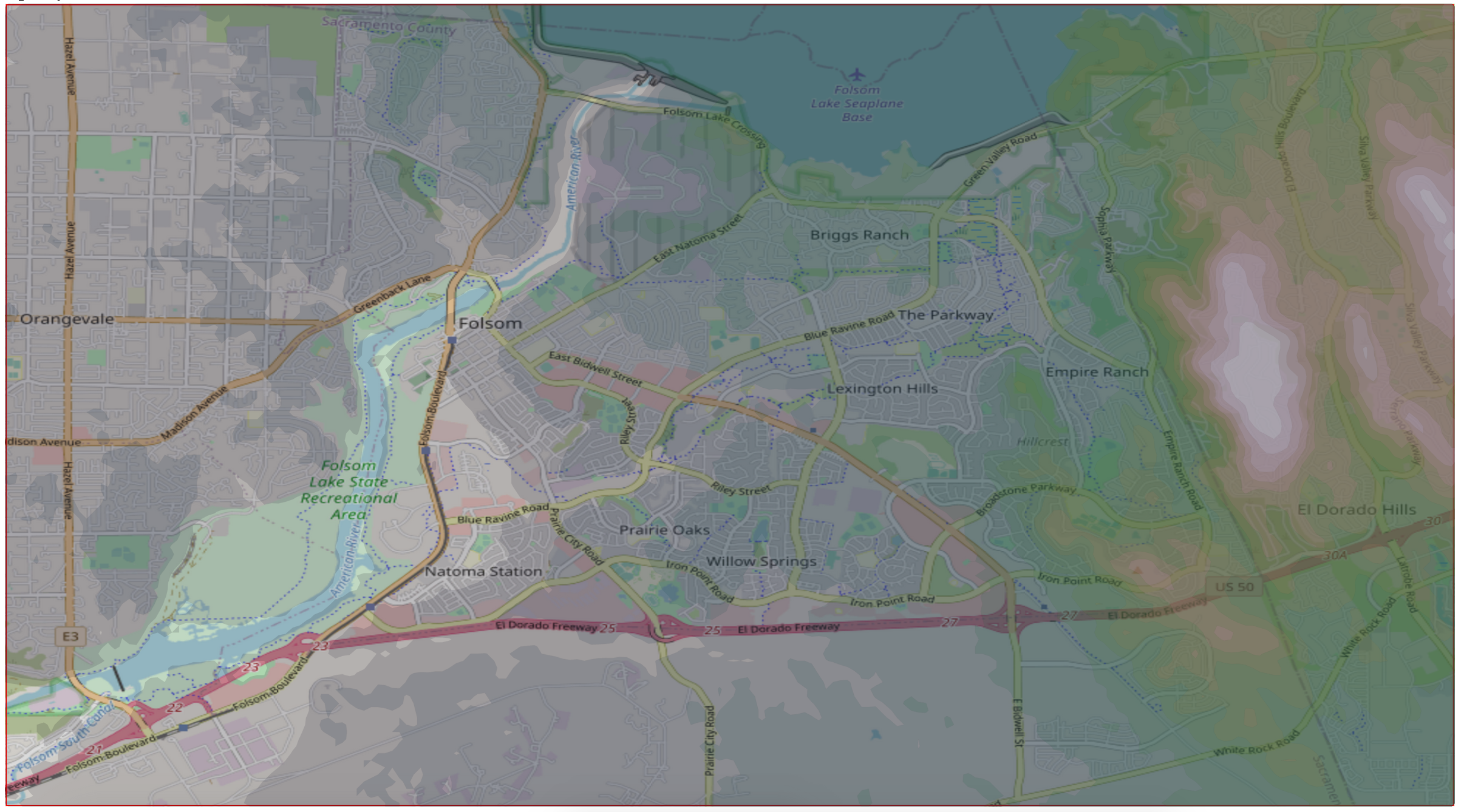
In my example, I also included a static image of the roads in my hometown under the contour plot and added a slider to adjust the opacity. Feel free to check out the example code for how those were implemented (right click on the page, and click “view page source”).

I collected some D3 mapmaking tips and tricks for anyone that wants to try their hand at making maps with D3, which I hope will help people create more cool maps and visualizations of open data.

DANNY YANG

about me · blog · projects · hire me