The heatmap is one of my favorite features in Strava. It’s fun to scroll through my personal heatmap and reminisce about adventures biking in other states and countries.
I’ve always wondered what that heatmap would look like for my Citi Bike rides. Unfortunately, the Citi Bike app doesn’t have this functionality - all it shows is how many stations I’ve visited and how many rides I’ve done.
In order to satisfy my curiosity, I had to take things into my own hands.
In this blog post, I’ll show you how I downloaded and visualized my Citi Bike ride history, showcasing several types of heatmaps and visualization techniques along the way. After that, I’ll also use the same techniques to visualize system-wide data, creating something akin to Strava’s Global Heatmap.
All the code for this blog post lives in this Github repository, if you want to try it for yourself. For those of you not living in NYC, don’t worry: this should work for all Lyft-operated bikeshare systems (SF, Chicago, DC, Boston, Portland, etc).
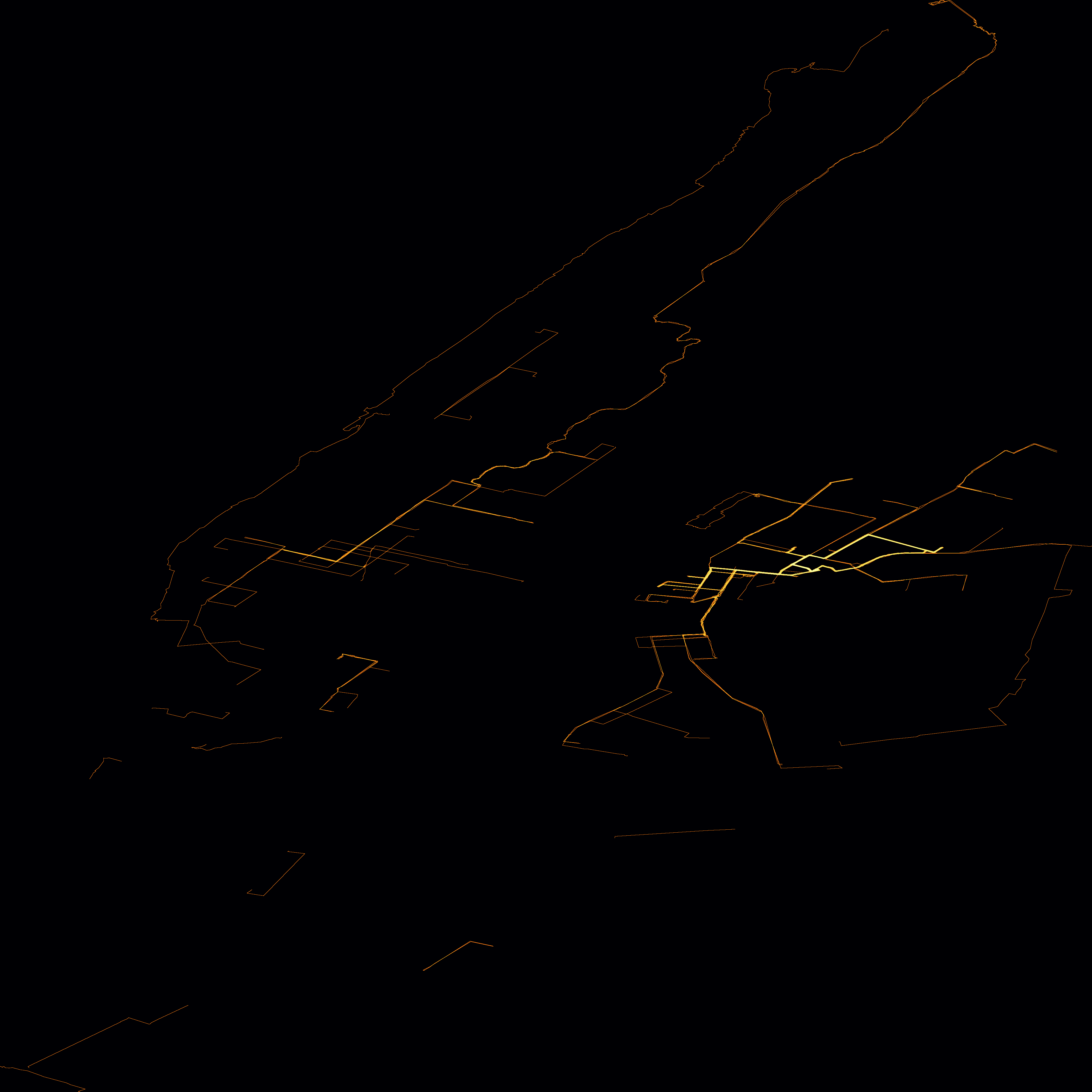
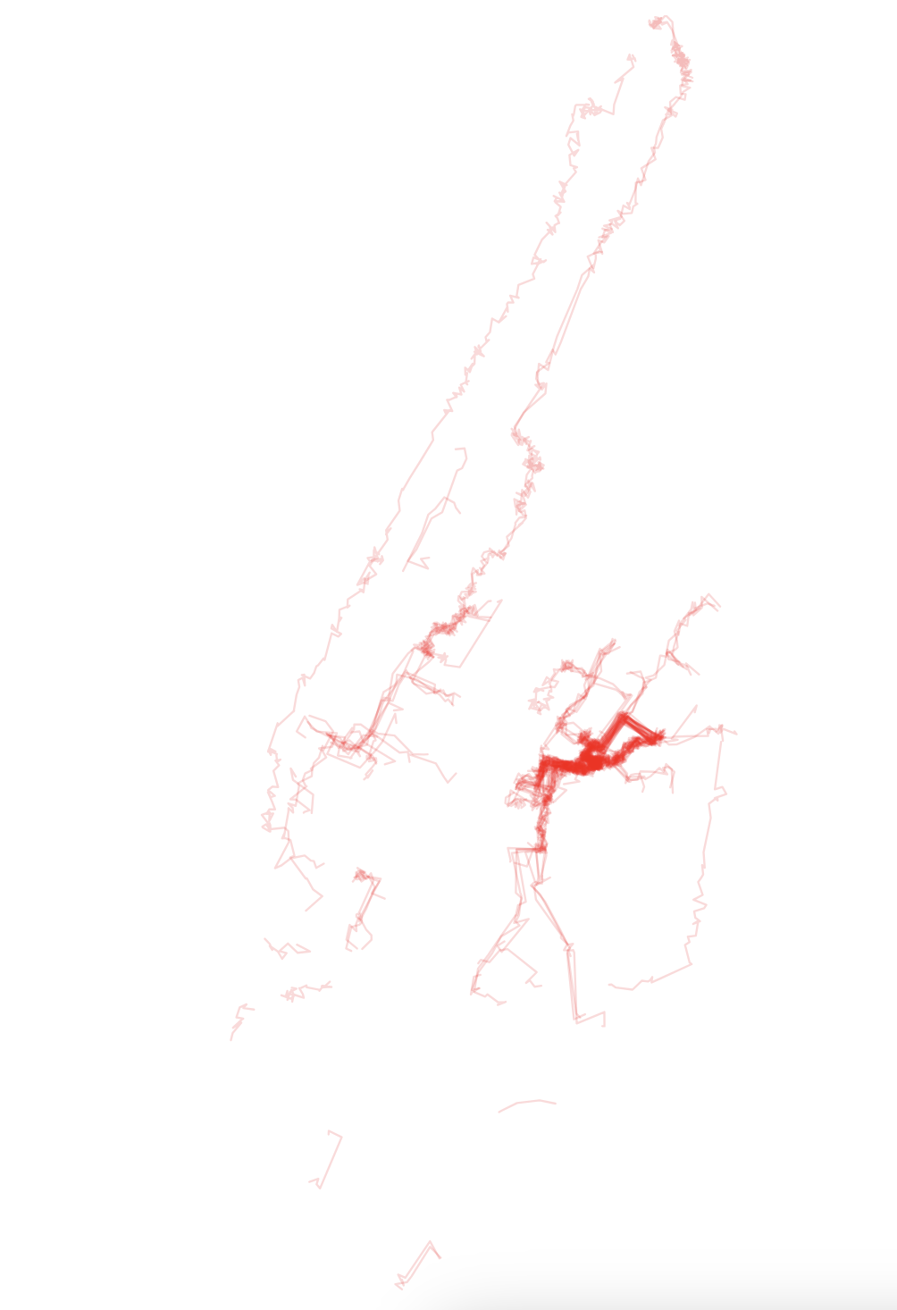
Before we get started, here’s a sneak peek of my personal heatmap:
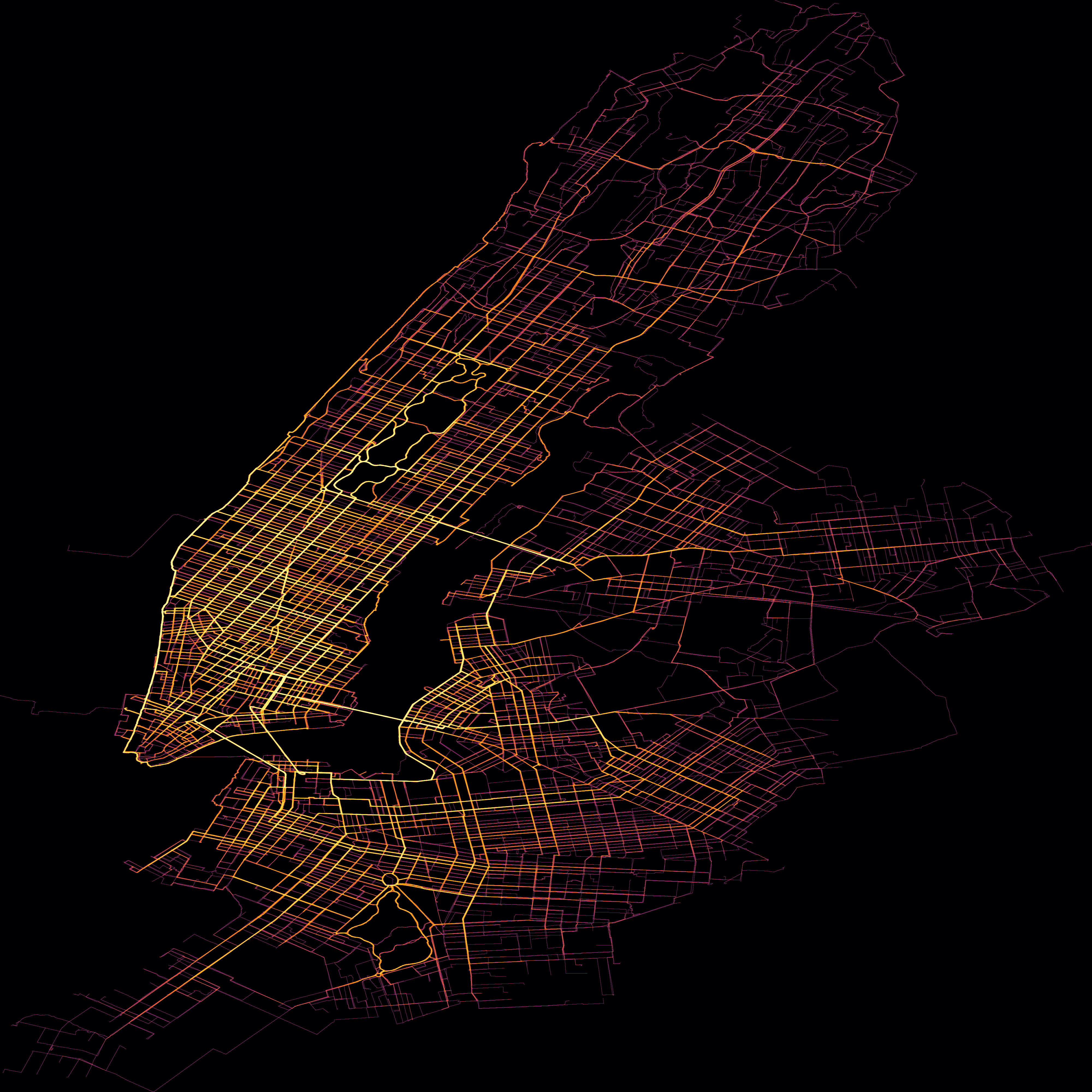
And here’s the system-wide heatmap:
Part 1: Personal Heatmap #
While Citi Bike provides useful system-wide data in its API, there is no official way to download your personal ride history from Citi Bike. Luckily, I found this script by fhoffa that scrapes the ride data from the Citi Bike website while you’re logged in.
While scripts of this sort tend to be brittle and may break if Lyft decides to change their website, I’m happy to say that I was able to use it to download all 200+ rides I’ve taken.
The data for a single ride looks something like this:
  {
    "rideId": "2172248736204432940",
    "startTimeMs": "1768070075146",
    "endTimeMs": "1768070435146",
    "price": {
      "formatted": "$0.00"
    },
    "duration": 360000,
    "rideableName": "361-0557",
    "startAddress": "Myrtle Ave & Marcy Ave",
    "endAddress": "Emerson Pl & Myrtle Ave",
    "lineItems": [
      {
        "title": "Free unlock",
        "amount": {
          "formatted": "$0.00"
        }
      }
    ]
  }
You’ll notice that there is a start and ending address (the names of the Citi Bike docks), but no data on the actual route between the docks. The fine-grained GPS data of e-bikes is not publicly available, and I’m pretty sure that the manual (“acoustic”, as some like to call it) bikes don’t have GPS at all.
In any case, the exact routes aren’t available, so I decided that Google Maps biking directions would be a good enough approximation of my route. First, I took each station pair and used the Citi Bike Station Information API to look up their coordinates. Then, I used the Google Maps Routes API to get a GeoJSON of the estimated route between the stations.
There were a couple of things to watch out for here:
- Citi Bike docks open and close all the time, so not every dock in my ride could be found in the Station Information API.
- If the ride starts and ends at the same station, there’s no way to guess the route. In some cases it might be obvious (like a lap of Prospect Park or Central Park), but I didn’t bother manually categorizing each one.
With Google’s best guesses for my routes retrieved, I could finally see what the data looked like.
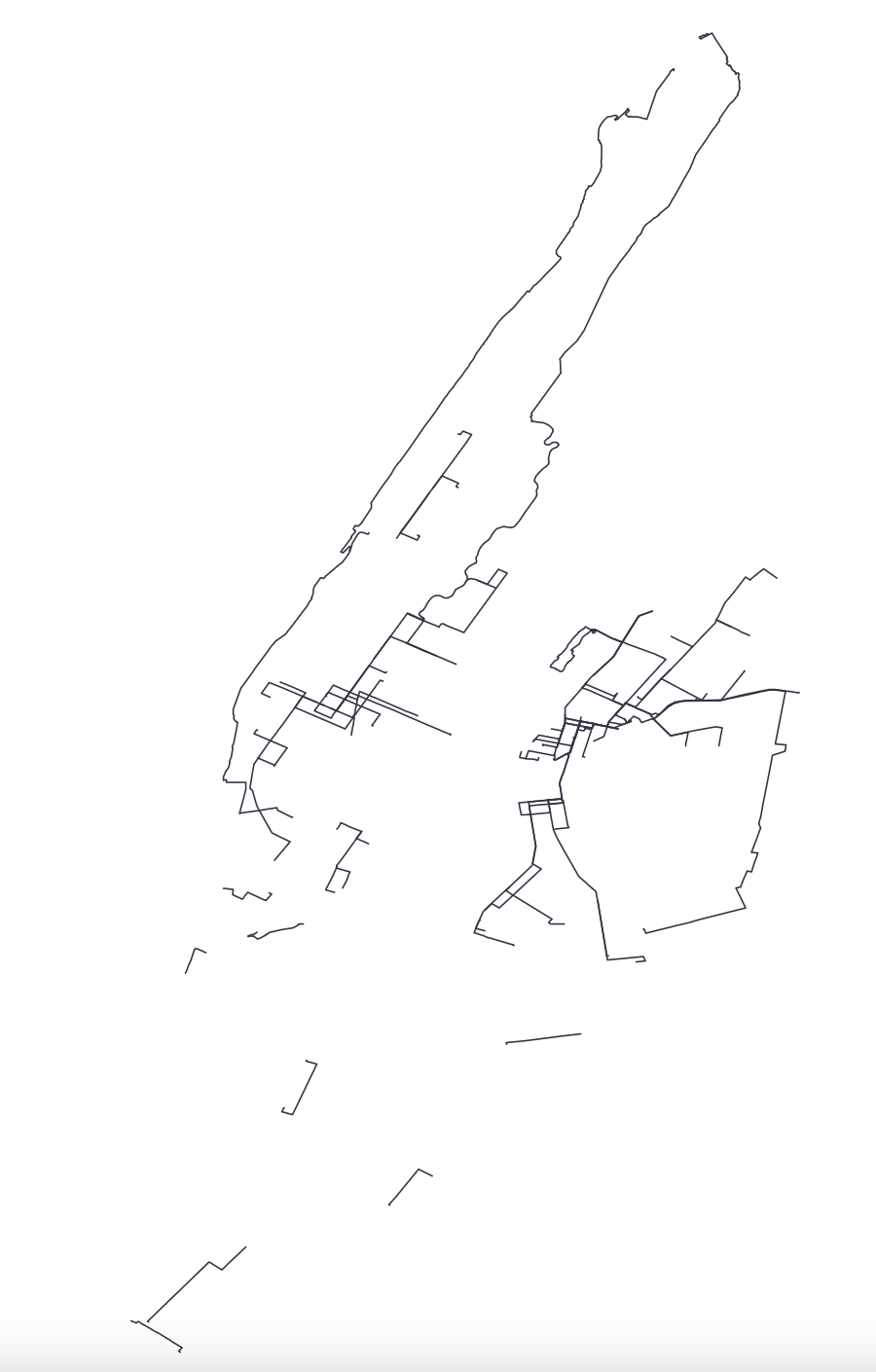
I immediately spotted the times I biked to the Cloisters, and things mostly looked pretty good! There were two issues I noticed as I looked closer:
- Google Maps doesn’t treat the bridge between Randall’s Island and Queens as a valid biking route, so even though I’ve taken a Citi Bike over the bridge before it doesn’t show up.
- The eastern route that meanders through Central Park to get to the Cloisters is wrong. It was during Summer Streets so I actually went up Park Ave, but Google had no way of knowing that.
It was interesting seeing a little bit of data/fidelity being lost at each step of the process, and this was certainly not the end of it.
Next, I wanted to view the data as a heatmap. An easy way to do this is to plot each line with a low opacity, overlapping lines will naturally appear darker. I threw together a quick implementation in D3.js and here’s what it looked like:
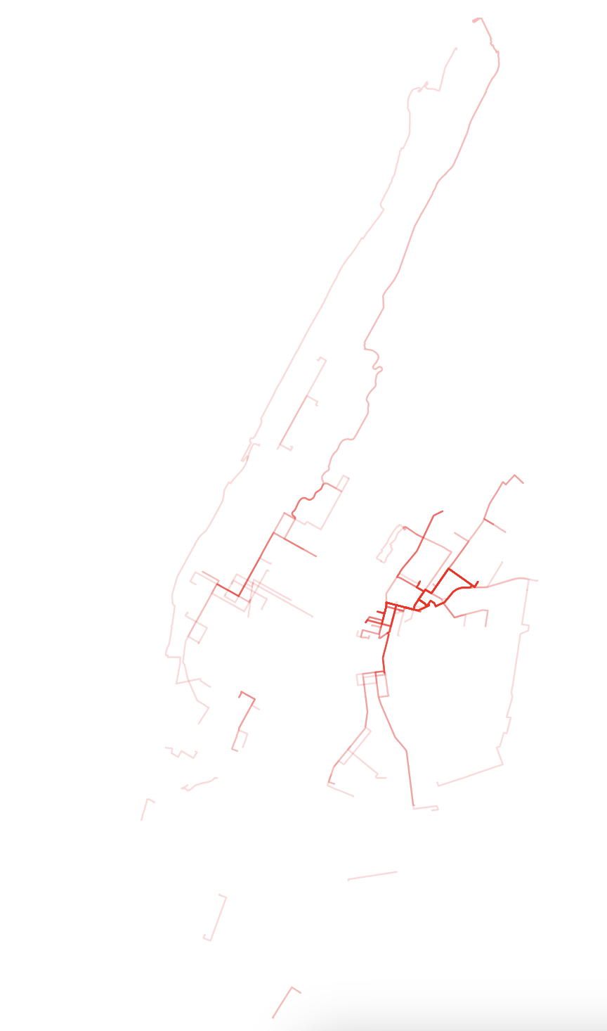
Pretty good, but compared to a Strava heatmap it looks a little too clean. Google Maps returns the biking directions as a straight lines down the center of the road, while Strava’s GPS tracking captures many more imperfections in your route - which lane you took, which cars you weaved around. This makes no two rides identical, and adds an organic look to the Strava heatmap that this one currently lacks.
There’s a technique to add noise to data visualizations called jittering - the idea is that we can add small random deviations to each coordinate in the line, to make them not overlap perfectly.
While reading up on Strava’s heatmap on their engineering blog, I learned that Strava still adds jitter to each GPS data point, because some devices snap your coordinate to the center of the road.
If even Strava was doing it, I decided that I had to fully embrace the imperfections in the process and intentionally degrade my data even more.
With a small amount of jitter applied, the lines look messier and closer to the aesthetic I’m aiming for.
The jitter worked better on the curved routes than the straight ones, because a perfectly straight line down an avenue has no lines to adjust other than the endpoints. One way to mitigate this is to synthesize points to break up the longer line segments, but I didn’t bother since I thought this was already good enough.
For fun, I decided to turn the jitter on each point up to 100 meters to see what it would look like. The end result was very fuzzy and abstract, and in my opinion quite pretty. It might be fun to make it into a poster and hang it up on the wall.
Thus far I’ve been using vector graphics, where the lines are perfectly straight and all the same color. To truly get something resembling the Strava heatmap, I would have to switch to a raster format, where the center of each line is a different color than the edges.
I wrote a quick script to generate a 4000x4000 raster image where each pixel is colored based on how many times a route intersects with it. Instead of building a color scale off of the raw values, I colored them based on the CDF (cumulative distribution function) - if a particular pixel’s value was greater than 90% of the other values, it would get the 90% color on the scale. This is the same technique Strava used in their heatmap.
I was very pleased with the end result:
Part 2: System-wide Heatmap #
I was curious to see how this would look as a “global” heatmap, using system-wide ride data. Citi Bike provides anonymized ride data on their website, approximately 400MB-1GB of data each month.
For the system-wide heatmap, I took a random sample of 10,000 rides from the October 2025 dataset. This limit was mainly due to constraints around the Google Maps API, which only allows 10,000 free requests per month.
First up is the vector heatmap:
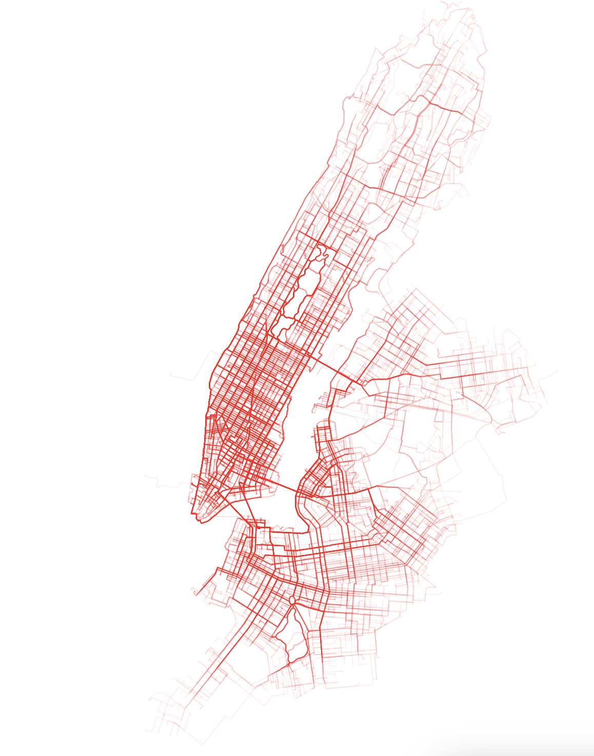
Of course, I had to turn the jitter up to max for this one too. I must say again, I really dig the look of this viz. It looks very organic, almost like blood vessels.
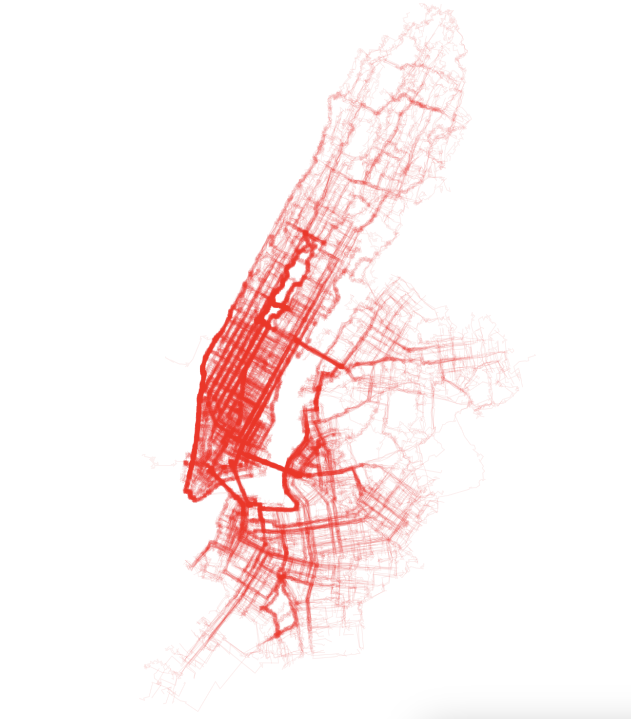
The raster heatmap looks like this:
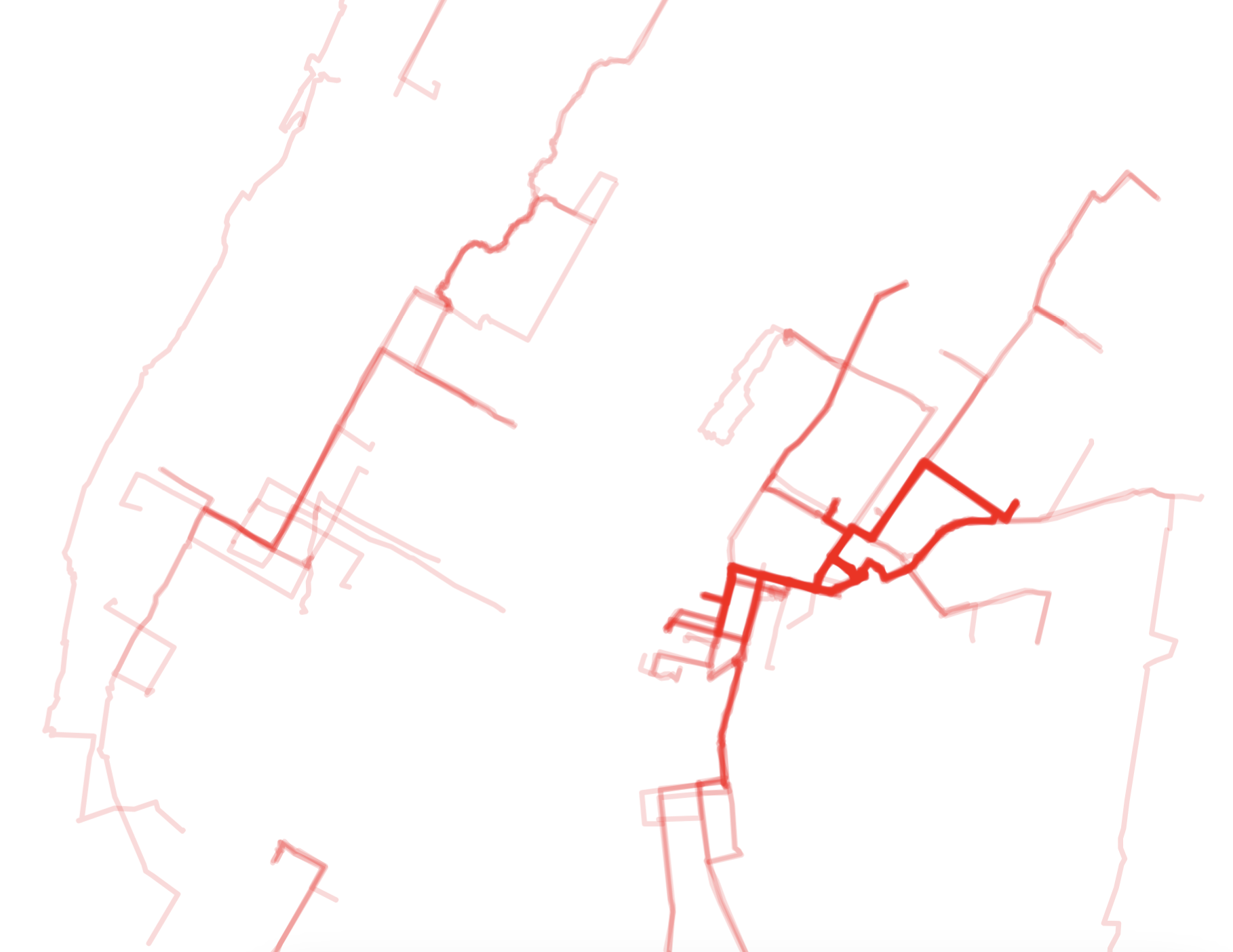
Here’s a zoomed-in view:
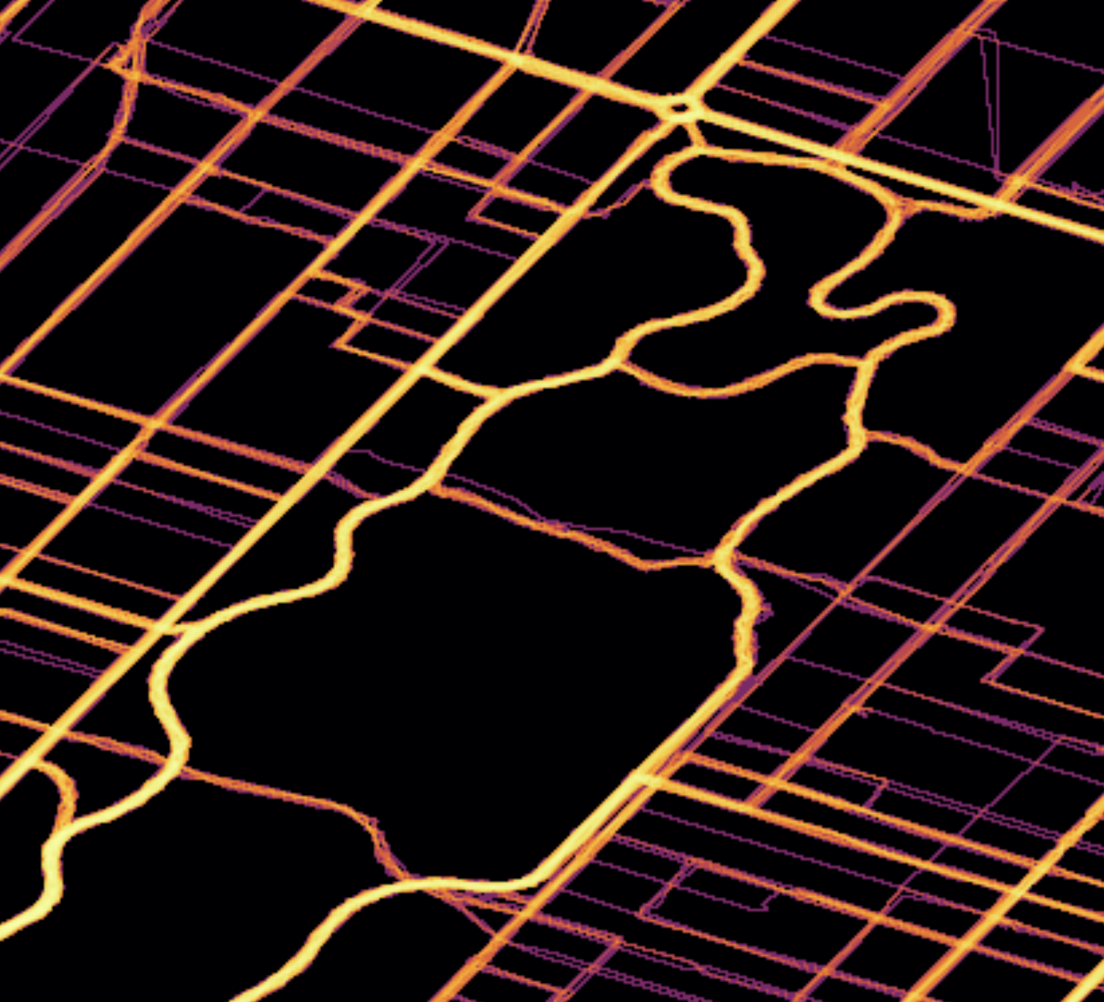
Looking at the larger map, 1st/2nd/3rd Aves in Upper East Side & crosstown routes north of Central Park are notable hot spots. These are all symptoms of the same problem - these areas are underserved by public transit, which forces more people to get around by bike. Luckily, the 2nd Ave Subway may alleviate these issues, especially with the newly-announced crosstown extension at 125th street. For 3rd ave specifically, the bicycle-friendly “green wave” traffic light timing may also be a factor.
Outside of Manhattan, Bushwick and Red Hook appear very bright. While both of those neighborhoods have subway access, the subway layout isn’t useful for getting around within the neighborhood, and many people live a long walk away from the nearest station. In Queens, the deeper parts of Astoria have a similar story, with a noticeable connections between the N/W and the M/R. The lack of crosstown subways in The Bronx is also very evident, with multiple bright east-west routes present on the map.
Conclusion #
This project was a fun exploration into techniques for visualizing route data as heatmaps. I got to satisfy a longstanding curiosity, and along the way I learned to embrace guessing, approximations, and adding intentional imperfections to my data in pursuit of a great visualization.
All the code for this blog post lives in this Github repository, so please feel free to try it out for yourself, and let me know what you come up with!
In the future, it would be awesome to reimagine this visualization as a physical installation, like this Reddit user. It wouldn’t be the first time I’ve done something like that.
Further Reading #
Other bikeshare systems have been mapped using similar techniques. Check them out!